
This work is licensed under a Creative Commons Attribution-ShareAlike 4.0 International License
The corresponding files can be obtained from:
- Jupyter Notebook:
buckling_3d_solid.ipynb - Python script:
buckling_3d_solid.py
Linear Buckling Analysis of a 3D solid
This demo has been written in collaboration with Eder Medina (Harvard University).
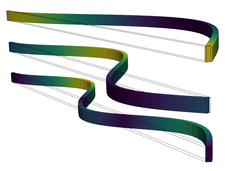
In this numerical tour, we will demonstrate how to compute the buckling modes of a three-dimensional elastic solid under a conservative loading. The critical buckling loads and buckling modes are computed by solving a generalized non-hermitian eigenvalue problem using the SLEPcEigensolver. This example is closely related to the Modal analysis of an elastic structure and the Eulerian
buckling of a beam demos. For more details on the theoretical formulation, the reader can refer to [NGU00].
Geometrically Nonlinear Elasticity
To formulate the buckling problem, we must consider a general geometrically nonlinear framework. More precisely, we will consider the case of small-strain/large displacements that are expected in typical buckling analysis.
We consider the Green-Lagrange strain tensor \(\be\) defined as:
Note that this can be rewritten in tensor format as
where we isolate the linear \(\beps(\bu)\) and nonlinear quadratic part \(\bq(\bu, \bu)=\nabla\bu\T\nabla\bu\).
Since we restrict to a small strain assumption, we adopt a standard linear Hookean behaviour for the material material model which can be described by the following quadratic elastic energy density:
where \(\mathbb{C}\) is the elastic moduli tensor.
We seek to find the underlying equilibrium displacement field \(\bu\) as a function of a scalar loading parameter \(\lambda\) under a set of prescribed external surface forces \(\bt(\lambda)\).
Equilibrium and stability conditions
Let us consider the total potential energy functional:
The equilibrium equations are obtained from the first variation which must vanish:
where \(\delta\bu\) is any kinematically admissible perturbation direction and where:
The stability conditions of an equilibrium are obtained from the Lejeune-Dirichlet theorem stating that the energy second variation must be positive. Here the second variation bilinear form is given by:
where:
Bifurcation point
A given equilibrium solution \(\lambda^c, \bu^c=\bu(\lambda^c)\) is a bifurcation point if the second variation vanishes for some \(\delta\bu\). \(\lambda^c\) defines the bifurcation load and \(\delta\bu\) the bifurcation mode. Hence, we have:
Linear buckling analysis
When performing a linear buckling analysis, we look for bifurcation points on the fundamental equilibrium branch obtained by a small displacement assumption. As a result, in the above bifurcation equation the quadratic contribution in the first term can be neglected and the Green-Lagrange strain \(\be(\bu^c)\) can be replaced by the linearized strain \(\beps(\bu^c)\). Besides, in the small-displacement assumption, if the loading depends linearly on the load parameter \(\lambda\), the small displacement solution also depends linearly on it. We therefore have \(\bu^c= \lambda^c\bu_0\) and the bifurcation condition becomes:
After, introducing the inital pre-stress \(\bsig_0 = \mathbb{C}:\beps(\bu_0)\), the last term can be rewritten as \(\bsig_0:\bq(\delta\bv,\delta\bu) = (\nabla \delta \bv) \bsig_0 (\nabla \delta\bu)\T\) so that :
We recognize here a linear eigenvalue problem where the first term corresponds to the classical linear elasticity bilinear form and the second term is an additional contribution depending on the pre-stressed state \(\bu_0\). Transforming this variational problem into matrix notations yields:
where \([\mathbf{K}]\) is the classical linear elastic stiffness matrix and \([\mathbf{K}_G(\bu_0)]\) the so-called geometrical stiffness matrix.
FEniCS implementation
Defining the Geometry
Here we will consider a fully three dimensional beam-like structure with length \(L = 1\) and of rectangular cross-section with height \(h = 0.01\), and width \(b = 0.03\).
[1]:
from dolfin import *
import matplotlib.pyplot as plt
import numpy as np

L, b, h = 1, 0.01, 0.03
Nx, Ny, Nz = 51, 5, 5

mesh = BoxMesh(Point(0, 0, 0), Point(L, b, h), Nx, Ny, Nz)
Solving for the pre-stressed state \(\bu_0\)
We first need to compute the pre-stressed linear state \(\bu_0\). It is obtained by solving a simple linear elasticity problem. The material is assumed here isotropic and we consider a pre-stressed state obtained from the application of a unit compression applied at the beam right end in the \(X\) direction while the \(Y\) and \(Z\) displacement are fixed, mimicking a simple support condition. The beam is fully clamped on its left end.
[2]:
E , nu = 1e3, 0.

mu = Constant(E/2/(1+nu))
lmbda = Constant(E*nu/(1+nu)/(1-2*nu))

def eps(v):
    return sym(grad(v))
def sigma(v):
    return lmbda*tr(eps(v))*Identity(v.geometric_dimension())+2*mu*eps(v)

# Compute the linearized unit preload
N0 = 1
T = Constant((-N0, 0, 0))
V = VectorFunctionSpace(mesh, 'Lagrange', degree = 2)
v = TestFunction(V)
du = TrialFunction(V)

# Two different ways to define how to impose boundary conditions
def left(x,on_boundary):
    return near(x[0], 0.)

def right(x, on_boundary):
    return near(x[0], L)

boundary_markers = MeshFunction('size_t', mesh, mesh.topology().dim()-1)
ds = Measure('ds', domain=mesh, subdomain_data=boundary_markers)
AutoSubDomain(right).mark(boundary_markers, 1)

# Clamped Boundary and Simply Supported Boundary Conditions
bcs = [DirichletBC(V, Constant((0, 0, 0)), left),
       DirichletBC(V.sub(1), Constant(0), right),
       DirichletBC(V.sub(2), Constant(0), right)]

# Linear Elasticity Bilinear Form
a = inner(sigma(du), eps(v))*dx

# External loading on the right end
l = dot(T, v)*ds(1)
We will reuse our stiffness matrix in the linear buckling computation and hence we supply a PETScMatrix and PETScVector to the system assembler. We then use the solve function on these objects and specify the linear solver method.
[3]:
K = PETScMatrix()
f = PETScVector()
assemble_system(a, l, bcs, A_tensor=K, b_tensor=f)

u = Function(V,name = "Displacement")
solve(K, u.vector(), f, "mumps")

# Output the trivial solution
ffile = XDMFFile("output/solution.xdmf")
ffile.parameters["functions_share_mesh"] = True
ffile.parameters["flush_output"] = True
ffile.write(u, 0)
Forming the geometric stiffness matrix and the buckling eigenvalue problem
From the previous solution, the prestressed state \(\bsig_0\) entering the geometric stiffness matrix expression is simply given by sigma(u). After having formed the geometric stiffness matrix, we will call the SLEPcEigenSolver for solving a generalized eigenvalue problem \(\mathbf{Ax}=\lambda \mathbf{Bx}\) with here \(\mathbf{A}=\mathbf{K}\) and \(\mathbf{B}=-\mathbf{K}_G\). We therefore include directly the negative sign in the definition of the geometric stiffness
form:
[4]:
kgform = -inner(sigma(u), grad(du).T*grad(v))*dx

KG = PETScMatrix()
assemble(kgform, KG)

# Zero out the rows to enforce boundary condition
for bc in bcs:
    bc.zero(KG)
The buckling points of interest are the smallest critical loads, i.e. the points corresponding to the smallest \(\lambda^c\).
We now pass some parameters to the SLEPc solver. In particular, we peform a shift-invert transform as discussed in the Eulerian buckling of an elastic beam tour.
[5]:
# What Solver Configurations exist?
eigensolver = SLEPcEigenSolver(K, KG)
print(eigensolver.parameters.str(True))
<Parameter set "slepc_eigenvalue_solver" containing 8 parameter(s) and parameter set(s)>

  slepc_eigenvalue_solver  |    type    value    range  access  change
  --------------------------------------------------------------------
  maximum_iterations       |     int  <unset>  Not set       0       0
  problem_type             |  string  <unset>  Not set       0       0
  solver                   |  string  <unset>  Not set       0       0
  spectral_shift           |  double  <unset>  Not set       0       0
  spectral_transform       |  string  <unset>  Not set       0       0
  spectrum                 |  string  <unset>  Not set       0       0
  tolerance                |  double  <unset>  Not set       0       0
  verbose                  |    bool  <unset>  Not set       0       0
[6]:
eigensolver.parameters['problem_type'] = 'gen_hermitian'
eigensolver.parameters['solver'] = "krylov-schur"
eigensolver.parameters['tolerance'] = 1.e-12
eigensolver.parameters['spectral_transform']  = 'shift-and-invert'
eigensolver.parameters['spectral_shift'] = 1e-2

# Request the smallest 3 eigenvalues
N_eig = 3
print("Computing {} first eigenvalues...".format(N_eig))
eigensolver.solve(N_eig)
print("Number of converged eigenvalues:", eigensolver.get_number_converged())

eigenmode = Function(V)

# Analytical beam theory solution
# F_cr,n = alpha_n^2*EI/L^2
# where alpha_n are solutions to tan(alpha) = alpha
alpha = np.array([1.4303, 2.4509, 3.4709] + [(n+1/2) for n in range(4, 10)])*pi
I = b**3*h/12
S = b*h

for i in range(eigensolver.get_number_converged()):
    # Extract eigenpair
    r, c, rx, cx = eigensolver.get_eigenpair(i)

    critical_load_an = alpha[i]**2*float(E*I/N0/S)/L**2
    print("Critical load factor {}: {:.5f} FE | {:.5f} Beam".format(i+1, r, critical_load_an))

    # Initialize function and assign eigenvector
    eigenmode.vector()[:] = rx
    eigenmode.rename("Eigenmode {}".format(i+1), "")

    ffile.write(eigenmode, 0)
Computing 3 first eigenvalues...
Number of converged eigenvalues: 3
Critical load factor 1: 0.16821 FE | 0.16826 Beam
Critical load factor 2: 0.49691 FE | 0.49405 Beam
Critical load factor 3: 0.98918 FE | 0.99084 Beam
Note that the analysis above is not limited to problems subject to Neumann boundary conditions. One can equivalenty compute the prestress resulting from a displacement control simulation and the critical buckling load will correspond to the critical buckling displacement of the structure.
References
[NGU00]: Nguyen, Q. S. (2000). Stability and nonlinear solid mechanics. Wiley.