This work is licensed under a Creative Commons Attribution-ShareAlike 4.0 International License

Reissner-Mindlin plate with Quadrilaterals

Introduction

This program solves the Reissner-Mindlin plate equations on the unit square with uniform transverse loading and fully clamped boundary conditions. The corresponding file can be obtained from reissner_mindlin_quads.py.

It uses quadrilateral cells and selective reduced integration (SRI) to remove shear-locking issues in the thin plate limit. Both linear and quadratic interpolation are considered for the transverse deflection \(w\) and rotation \(\underline{\theta}\).

Note

Note that for a structured square grid such as this example, quadratic quadrangles will not exhibit shear locking because of the strong symmetry (similar to the criss-crossed configuration which does not lock). However, perturbating the mesh coordinates to generate skewed elements suffice to exhibit shear locking.

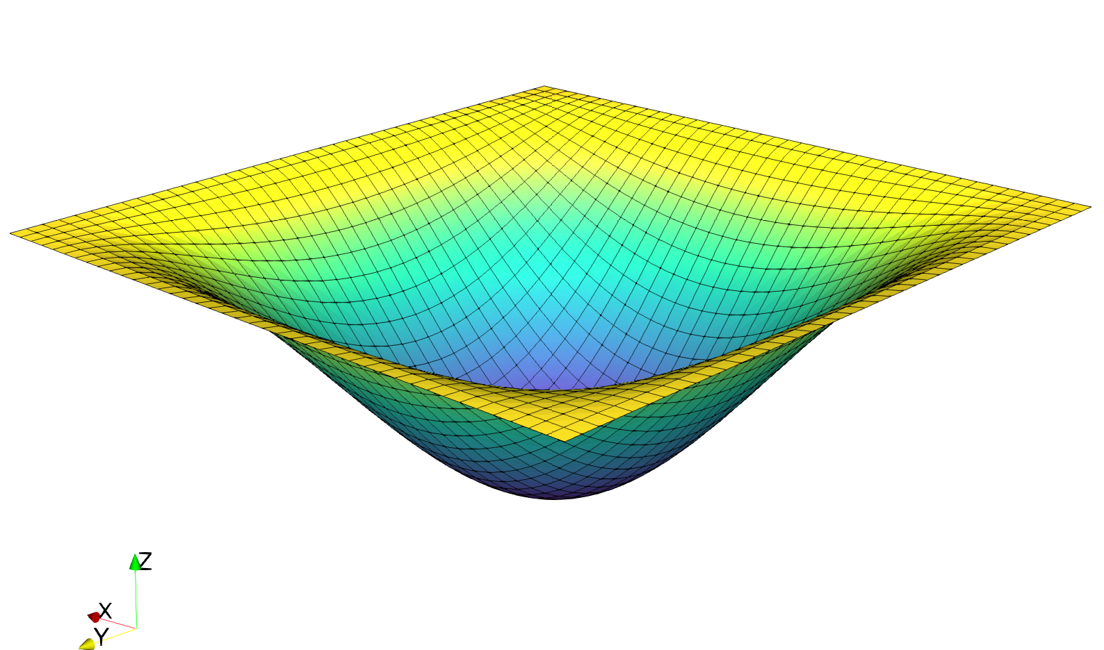
The solution for \(w\) in this demo will look as follows:

Implementation

Material parameters for isotropic linear elastic behavior are first defined:

from dolfin import *

E = Constant(1e3)
nu = Constant(0.3)

Plate bending stiffness \(D=\dfrac{Eh^3}{12(1-\nu^2)}\) and shear stiffness \(F = \kappa Gh\) with a shear correction factor \(\kappa = 5/6\) for a homogeneous plate of thickness \(h\):

thick = Constant(1e-3)
D = E*thick**3/(1-nu**2)/12.
F = E/2/(1+nu)*thick*5./6.

The uniform loading \(f\) is scaled by the plate thickness so that the deflection converges to a constant value in the thin plate Love-Kirchhoff limit:

f = Constant(-thick**3)

The unit square mesh is divided in \(N\times N\) quadrilaterals:

N = 50
mesh = UnitSquareMesh.create(N, N, CellType.Type.quadrilateral)

Continuous interpolation using of degree \(d=\texttt{deg}\) is chosen for both deflection and rotation:

deg = 1
We = FiniteElement("Lagrange", mesh.ufl_cell(), deg)
Te = VectorElement("Lagrange", mesh.ufl_cell(), deg)
V = FunctionSpace(mesh, MixedElement([We, Te]))

Clamped boundary conditions on the lateral boundary are defined as:

def border(x, on_boundary):
    return on_boundary

bc =  [DirichletBC(V, Constant((0., 0., 0.)), border)]

Some useful functions for implementing generalized constitutive relations are now defined:

def strain2voigt(eps):
    return as_vector([eps[0, 0], eps[1, 1], 2*eps[0, 1]])
def voigt2stress(S):
    return as_tensor([[S[0], S[2]], [S[2], S[1]]])
def curv(u):
    (w, theta) = split(u)
    return sym(grad(theta))
def shear_strain(u):
    (w, theta) = split(u)
    return theta-grad(w)
def bending_moment(u):
    DD = as_tensor([[D, nu*D, 0], [nu*D, D, 0],[0, 0, D*(1-nu)/2.]])
    return voigt2stress(dot(DD,strain2voigt(curv(u))))
def shear_force(u):
    return F*shear_strain(u)

The contribution of shear forces to the total energy is under-integrated using a custom quadrature rule of degree \(2d-2\) i.e. for linear (\(d=1\)) quadrilaterals, the shear energy is integrated as if it were constant (1 Gauss point instead of 2x2) and for quadratic (\(d=2\)) quadrilaterals, as if it were quadratic (2x2 Gauss points instead of 3x3):

u = Function(V)
u_ = TestFunction(V)
du = TrialFunction(V)

dx_shear = dx(metadata={"quadrature_degree": 2*deg-2})

L = f*u_[0]*dx
a = inner(bending_moment(u_), curv(du))*dx + dot(shear_force(u_), shear_strain(du))*dx_shear

We then solve for the solution and export the relevant fields to XDMF files

solve(a == L, u, bc)

(w, theta) = split(u)

Vw = FunctionSpace(mesh, We)
Vt = FunctionSpace(mesh, Te)
ww = u.sub(0, True)
ww.rename("Deflection", "")
tt = u.sub(1, True)
tt.rename("Rotation", "")

file_results = XDMFFile("RM_results.xdmf")
file_results.parameters["flush_output"] = True
file_results.parameters["functions_share_mesh"] = True
file_results.write(ww, 0.)
file_results.write(tt, 0.)

The solution is compared to the Kirchhoff analytical solution:

print("Kirchhoff deflection:", -1.265319087e-3*float(f/D))
print("Reissner-Mindlin FE deflection:", -min(ww.vector().get_local())) # point evaluation for quads
                                                                        # is not implemented in fenics 2017.2

For \(h=0.001\) and 50 quads per side, one finds \(w_{FE} = 1.38182\text{e-5}\) for linear quads and \(w_{FE} = 1.38176\text{e-5}\) for quadratic quads against \(w_{\text{Kirchhoff}} = 1.38173\text{e-5}\) for the thin plate solution.